 |
 |
- Search
| J Audiol Otol > Volume 22(3); 2018 > Article |
|
Abstract
The hearing-aid transducer is ubiquitous in the hearing-aid industry. For example, the balanced armature receiver (BAR), first invented by A.G. Bell, has been used in all telephone earphones because it has the highest output and best frequency response. Nevertheless, previous electro-mechanical studies on these miniature speakers are quite primitive, given the price of the transducers. Thus, more detailed analysis is critically important for the field of hearing science. This review study was motivated by HuntŌĆÖs parameter calibration (1954), a widely used commercial hearing-aid receiver (ED series, manufactured by Knowles Electronics, Inc.). In the body of the study, the transfer function of the BAR system (i.e., pressure over voltage) was calculated from HuntŌĆÖs parameters, solely from the electrical terminals of the device. The computed transfer function was then further investigated by comparing to the pole-zero fitting method using the methods of Gustavsen and Semlyen (1999) and Prony (1975). Based on our short experiment, the better fitting result was achieved with Gustavsen and SemlyenŌĆÖs method. By decomposing results of the transfer function fitting into all-pass and minimum-phase parts, the system was confirmed as a delay system. We conclude that the BAR system is linear, time-invariant, stable, and causal while providing an evidence-based understanding of the hearing-aid receiver system.
In general, a hearing-aid consists of three parts: a microphone (picks up sound), an amplifier (transforms sound into different frequencies, filters noise, and selectively amplifies each frequency region based on the difference in individuals with hearing loss via multi-band compression), and a receiver (sends the processed signal from the amplifier into the ear). A better understanding of each component of the hearing-aid can improve its sound quality. In this review paper, we analyze the hearing-aid receiver, which is one of the most important, expensive, and complex components of the hearing-aid; specifically, we study the balanced armature receiver (BAR), which converts an electrical signal (current) into acoustical pressure (or force in the case of an electro-mechanical system). In particular, while introducing a unique analysis procedure for the BAR system, the entire study can be summarized into three parts: 1) calculating the systemŌĆÖs transfer function from HuntŌĆÖs parameters, 2) pole-zero fitting of the transfer function, and 3) decomposition of the transfer function into all-pass and minimum-phase parts. This concept is inspired by Robinson, et al. [1], who approximated the length of the ear canal using the human earŌĆÖs reflectance data.
Beyond HuntŌĆÖs classic study [2], several papers have implemented anti-reciprocity in their electro-magnetic transducer model. In 2013, Kim and Allen [3] suggested a two-port anti-reciprocal network model of the BAR having a semiinductor, a gyrator (two poorly understood elements of special interest in the electro-magnetic transducer), and a pure delay. Their two-port impedance matrix is based on the classical expression of either Wegel [4] or Hunt [2] to transform electrical to acoustic segments,
where E is the voltage, I is the current, P is the pressure, and U is the volume velocity; the directions of I and U are defined as going into the network.
Note that s = Žā + jŽē, and
The transduction functions, Tea(s) and Tae(s), show anti-reciprocal characteristics of the system. For example, under the DC status (ignoring acoustic components), the systemŌĆÖs electro-magnetic coupling coefficient is a constant, -Tea = Tae = -Ta = B0l where B0 and l are the DC magnetic field and length of wire, respectively. The Tea(s) and Tae(s) have the same magnitudes but opposite signs.
Along with Eq. 1, the two-port electro-mechanic transducer equation can alternatively be represented in ABCD (a.k.a. transmission matrix) form, as given by
Here A, B, C, and D are functions of s to show that they are causal and complex analytic system variables. The signal variables E, I, P, and U, on the other hand, are functions of Žē, indicating they are signals and therefore neither causal nor analytic.
The fundamental difference between the two matrix representations lies in the coupling of acoustic and electric segments. Specifically, the electrical input parameters E and I are on the left side of the network (Eq. 6) and expressed in terms of the acoustical variables, P and U, on the right side of the network, via the four frequency-dependent parameters A, B, C, and D. Conversion between Eq. 1 and Eq. 6 yields the following relationships:
where ΔZ=ZeZa-TeaTae. Note that if C=0, Z does not exist.
Using a friendly approach, this paper is organized into four sections: First section introduces the theoretical background. The second section includes the pole-zero fitting algorithm and its derivation. In third and fourth sections, we present the experimental methods and their results, respectively. Conclusion is followed by the final section.
This section introduces the most critical theories and concepts needed to appreciate this study. These include concepts such as two-port network postulates and transfer functions with equivalent forms.
The impedance matrix representation of two-port networks (Eq. 1) is the matrix version of OhmŌĆÖs law. Like the one-port Thevenin/Norton model, the matrix system can characterize and generalize linear transducers [2,4,5]. Carlin and Giordano [6] summarized two-port networks in terms of six postulates: 1) Linearity (vs. nonlinearity)ŌĆĢA system obeys superposition. 2) Time-invariance (vs. time-variance)ŌĆĢA system does not depend on the time of excitation. 3) Passivity (vs. active)ŌĆĢThis addresses the conservation of energy law; a system cannot provide more power than the supplied amount. 4) Causality (vs. non-causality vs. anti-causality)ŌĆĢA system response cannot be affected by a future response. 5) Real-time function (vs. complex-time function)ŌĆĢThe systemŌĆÖs time response is real. 6) Reciprocity (vs. non-reciprocity vs. anti-reciprocity)ŌĆĢThe two transfer impedances (the two off-diagonal components) of the systems impedance matrix must be equal to be a reciprocal system. The anti-reciprocal network swaps the force and the flow, but one variable changes to the opposite direction.
Based on a study of McMillan [7] and Hunt [2], a moving-armature electro-magnetic transducer can be approximately considered to be a linear, time-invariant, passive, causal, real-time, and anti-reciprocal system (the off-diagonal elements if Eq. 1 has opposite signs). Therefore, this system is linear time-invariant (LTI) and capable of being analyzed using Laplace and Fourier transforms. In transform domains, the linear differential equations of the system (in the time domain) become linear and algebraic, so we can compute the algebra to study the LTI system. The linearity is the most important concept in the system theory. Many practical engineering systems can be designed as linear. This concept allows for easier and more convenient methods of system analysis and modeling. Time-invariance, as discussed above, means that if the same input is applied at different times, the output produced will be identical in shape and size but will be shifted in time.
If the input to an LTI system is x(t)=╬┤(t),
where y(t) is the output signal and h(t) is the systemŌĆÖs impulse response in the time domain. The Laplace transform of the input is X(s) =1, and the corresponding output yields
Eq. 9 can be rewritten as
The Laplace transform of h(t) is H(s), which is called the transfer function of the system with the complex frequency s=Žā+jŽē.
Using properties of the Laplace transform (linearity and derivative properties) yields
Eq. 10 can be found as the ratio of two polynomials,
One can see that the input coefficients are related to the numerator terms in H(s), and the output coefficients determines the denominator of H(s).
H(s) can be factored into first-order terms in s,
where K is the scale factor. The s values, which make H(s) zero (s=ni) and infinity (s=dk), are called the systemŌĆÖs zero and pole, respectively.
Moreover, a partial fraction of H(s) with a residual can be achieved by using the vector fitting procedure [8],
where pm is pole and rm is residual; d and e are real values, whereas pm and rm can be either real or complex values. If e is zero, then the number of poles and zeros in the system is the same.
The LTI systemŌĆÖs stability can be discussed via the impulse response, the transfer function, and the systemŌĆÖs poles and zeros. In terms of the region of convergence (ROC), the imaginary axis of the s-plane is included in ROC for a stable system. Specifically, for the system to be stable, all poles are in the left half plane (LHP) in a causal system case, whereas all poles must be in the right half plane (RHP) in an anti-causal system case (see the Table 1).
A data fitting process is required to examine the experimental data in systematic ways. Gustavsen and SemlyenŌĆÖs [8] and PronyŌĆÖs [9] algorithms are employed in this study to analyze our physical system, the BAR. The comparison using two methods for our system is discussed here.
Gustavsen and Semlyen [8] introduce the vector fitting procedure. This method is also called pole-fitting or rational approximation. Assuming that we have data F(s), the aim is to find all Ri, Qi, D, and E in a residual expansion of the form F ^
It is important to note that in our study, the data are only available as a function of Žē; thus, we can rewrite the data F(s) as F(Žē), which is related to the fitted function F ^ F ^
As an initial step, the explicit algebraic expression of Žā(s) and Žā┬ĘF ^
(Žā┬ĘF ^
Once we estimate the values of pi, bi, e, and d in Eq. 17, the equation can be redefined as a product form
Therefore, our fitting function F ^
Thus, the zeros of the scaling function Žā(s) (zi in Eq. 19) become the poles of the model function F ^ F ^ F ^ F ^
This algorithm is implemented by the method of Gustavsen and Semlyen [8], while applying for function rationalfit.m of the MATLAB (MathWorks, Inc., Washington DC, USA). This is a reasonable way to automate a fitting to within a given error tolerance. To facilitate an understanding of this algorithm, the procedure of this function is briefly explained as follows: Starting from the initial pole, the algorithm increases the order of the poles and searches for the best fit until the fit reaches the specified error tolerance level. An appropriate selection of starting poles is necessary for the convergence of the vector fitting method. For data with a resonance peak in magnitude (i.e., our data), Gustavsen and Semlyen [8] suggested that the complex conjugate pairs of the starting poles should be linearly distributed to achieve the best fitting result. Differences between the starting poles and the fitted poles can cause discrepancies between Žā(s) and (Žā┬ĘF ^
As the complex conjugate pairs of poles qi (Eq. 19) order changes, they converge to the true poles. Then the scaling function Žā(s) will become 1, meaning that the calculated zeros zi of Žā(s) have values arbitrarily close to the values of the starting poles, qi. This single process can iterate over the dataŌĆÖs frequency range until the fitting reaches the best fit. When it returns R F ^
One can also define the e and d values as initial conditions in that they affect the total number of fitted zeros, namely, Nz. For example, Nz is the same as the number of poles (N) when e is zero but d is not zero. If e and d are zero, we can have one fewer zeros than the poles because the numerator order is one less than the denominator (see Eq. 17). Similarly, when d and e are both nonzero, Nz is N+1. In this study, we use the fitting condition with e zero and d nonzero, allowing us the same number of poles and zeros. We reach a slightly different fitting result by varying the initial value of e and d, but this does not critically affect the overall performance of the fitting result. Eventually, when this augmented equation is fitted to the given data F(Žē) iterating toward Žā(s)=1, the order of the poles for the fitting function meets the given error tolerance. The error is calculated using a mean squared error (MSE), in decibels, relative to the L2 norm of the signal:
Eq. 21 returns one single number (total error, not varying frequency) to evaluate goodness of fit. Note that in our study, we allow an MSE tolerance of -30 dB, which corresponds to a root mean square relative error of 3.16%.
Another popular data fitting procedure used in this study is called the Prony method (PM) (developed by de Prony in 1795) [9]. It models data as a linear combination of exponentials. However, the performance of the PM is known to be poor when the data contain noise [10]. This method returns a large biased result due to the noise; for example, it fits exponentials to any additive noise present in the signal so that the damping terms become much greater than the actual values [10]. To derive the mathematical formulation for the original Prony analysis, we can define a fitting function, y ^
which is the sum of complex damped sinusoids, where Ai, Žāi, Žåi, and fi are amplitude, damping coefficient, phase, and frequency of component i, respectively. Also, L is the total number of the damped exponential components. This function estimates given data y(t), which consists of N samples y(tk)=y[k], where k=0, 1, 2, ..., N-1 are evenly spaced.
Via the Eulers theorem, the cos(2ŽĆfit+Žåi) term can be rewritten as a sum of exponentials:
where C i = A i 2 e jŽå i ╬╝ i = e ( Žā i + 2 jŽĆf i ) T
The PM searches for the Ci and ╬╝i in three steps: First, it solves the linear prediction model, which is constructed by the observed data set. Second, it finds roots of characteristic polynomials formed from the linear prediction coefficients. Third, it solves the original set of linear equations to obtain estimates of the exponential amplitude and sinusoidal phase.
Based on these concepts, in this study we have utilized MATLABŌĆÖs built-in function prony.m to execute the Prony analysis. This function is for the time-domain design of infinite impulse response filters. It models a signal by employing a user-specified order of poles and zeros. In our study, we use the same numbers of poles and zeros (14 for each) taken from GaustavsenŌĆÖs previous fitting results to compare the two fitting results. The PM assumes that frequencies are not periodic, which means they are not a sum of harmonically related sinusoidals. If we want to fit irrational data, we can use the Prony algorithm. For example, if we want to add two irrational sine waves [such as sin(ŽĆ) and sin(ŽĆ
The electrical input impedance measurement method [3] that is used to calculate HuntŌĆÖs parameters (Eqs. 2-5) is discussed here. Then we explain an explicit way to compute the transfer function from HuntŌĆÖs parameters. The pole-zero fitting result of the transfer function is discussed at the end of this section.
The electrical input impedance measurement method and data have been adapted from Kim and Allen [3] to compute HuntŌĆÖs parameters of the BAR as functions of the frequency. The chirp signal has been generated via MATLAB software on a laptop and sent to the BAR. The receiver has been maintained in the series position with a known value resistor such as 1 k╬® which source is grounded. Then the electrical input impedance Zin has been computed based on OhmŌĆÖs law. The signal-to-noise ratio is enhanced by averaging the response over more than 10 consecutive frames, and the first response block is dropped to consider the steady-state response.
In Kim and Allen [3] work, seven acoustic loads (different lengths of tubes including the no-load condition) are used for the measurement and seven corresponding electrical input impedance results are saved. The tube lengths are 0.2540, 0.3785, 0.8839, 1.2497, 2.3927, and 3.0658 cm. The same type tube is used with 0.15 cm of inner diameter, which is similar to the outer diameter of the BAR acoustic port (see the Fig. 7 of previous work from Kim and Allen [3]). Following Weece and Allen [11], a mathematical formation of measured Zin using Hunt parameters (Eqs. 2-5) is
where the acoustic load impedance ZL is
For the blocked-end tube indicating U=0, ZLŌēłZ0 coth (a┬Ętube length) where Z0 and a are the characteristic impedance of a tube and the complex propagation function, respectively. They are computed considering the viscous and thermal losses by Keefe [12] for calculation c=334.8 m/s, assuming 20┬░C room temperature.
Zin is sensitive to the acoustic load conditions; thus, each condition of Zin can be denoted as Zin|A, Zin|B, ..., Zin|F excluding the no-tube condition. There are three unknowns (Hunt parameters) in Eq. 25; to compute one set of unknowns, three conditions of Zin must be selected. The specific computation of the Hunt parameters using three input impedances is explained in Weece and Allen [11] and Kim and Allen [3].
Three cases of Zin in the BAR are randomly chosen to calculate the Hunt parameters (please see a Fig. 11 of the published paper by Kim and Allen [3]). Hunt parameters explain the intrinsic characteristics of the system; thus, calculating Hunt parameters is one way to calibrate the system. By manipulating these data, the systemŌĆÖs transfer function is computed as described in the next section.
The transfer function, H(Žē), of the system is calculated from HuntŌĆÖs parameters and is compared with the direct pressure measurement data. There is reasonable agreement among these measures up to 6-7 kHz. The mathematical definition of H(Žē) from HuntŌĆÖs parameter is pressure over voltage (P/E) with a zero volume velocity (U=0),
Note that this is the transduction impedance (one of HuntŌĆÖs parameters), while Thevenin pressure over voltage in Eq. 27 is defined as the transfer function of this system. The dark-green line in Fig. 1 is taken from the pressure measurement using an ER-7C probe microphone (Etymotic Research, Inc., Elk Grove Village, IL, USA) as real-world reference data. To compute H(Žē), the pressure data are divided by the input voltage (Ein) across the two electrical terminals of ED7045 (Knowles, Itasca, IL, USA) (U=0). Other than this direct pressure measurement, all responses are derived from the Hunt parameter calculation, using the electrical input impedance measurements data with various acoustical loads.
The two vector fitting procedures are performed using GustavsenŌĆÖs and PronyŌĆÖs methods. As discussed earlier, the former method provides a better data fitting result (shown in Fig. 2, 3). To compare the goodness of each method, we calculate each error measured across frequencies,
where f is frequency. In Fig. 4, we can observe high error rates in low frequencies and minimum error rates at the peak amplitude (resonance) of the data for both fitting methods. Overall lower error rates are observed in GustavsenŌĆÖs fitting results. For this study, therefore, we choose the better result data for further analysis.
We limit the fitting frequency range up to 6 kHz, where H(Žē) data start to show noise. The fitting result reflects reasonable agreement with the data within the frequency region of our interest (Fig. 2).
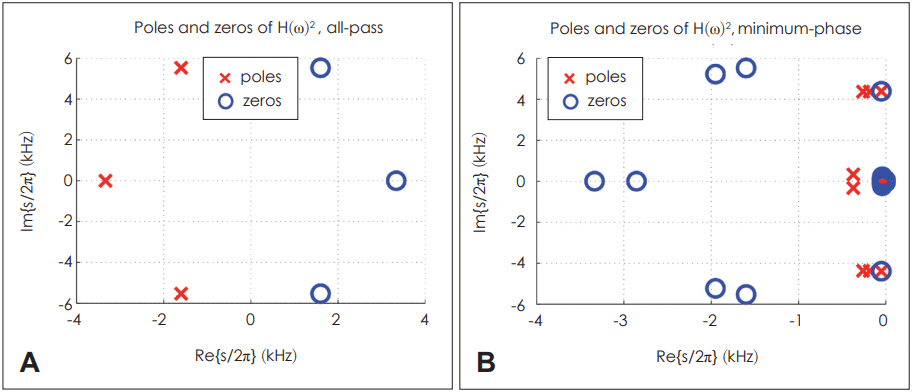
Due to the ŽĆ jump of H(Žē)ŌĆÖs phase in Fig. 1, the fitting results of H(Žē)2 are much better than those of H(Žē). Thus, H(Žē)2 is used as our fitting data. The ŽĆ jump happens during the HuntŌĆÖs parameter calculation procedure in MATLAB programming when computing Ta from T2. As a result, we can expect double poles and zeros for H(Žē)2 compared to H(Žē), but this does not affect the system analysis as the double poles and zeros are on top of each other. Fig. 5 shows the pole-zero plot of H(Žē)2.
Poles and zeros on the jŽē axis in Fig. 5 are on top of each other, meaning that they can cancel each other out. In this pole-zero fitting procedure, all poles are forced to be in LHP to keep the result stable; therefore, the region of convergence can be on the right side of the s-plane from the right-most pole location including the jŽē axis.
A causal stable filter, H(Žē), can be factored into a causal stable all-pass part cascading with a minimum-phase part,
where HAP(Žē) and HMP(Žē) are an all-pass filter and a minimum-phase filter, respectively. Without changing the amplitude of the original filter, H(Žē), the maximum-phase zeros in RHP of H(Žē), are reflected in LHP to compose HMP(Žē), whereas HAP (Žē) has the original maximum-phase zero (Fig. 6).
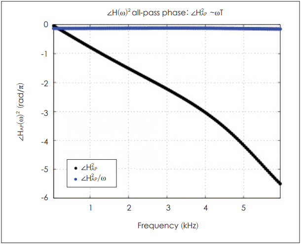
A lossless all-pass filer, HAP(Žē), has a frequency response where the magnitude is always 1,
where HAP(Žē)=Žå(Žē). Based on Fig. 7, we can approximate Žå(Žē)=ŽēT, yielding
where 2T=2Žå(Žē)/Žē is a constant.
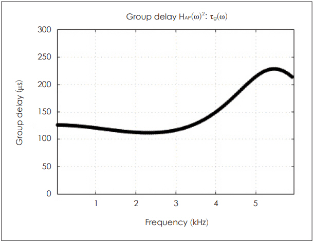
The group delay Žäg(Žē) of HAP(Žē)2 can be calculated as follows:
The result is shown in Fig. 8.
If one part of an entire system is approximated to be lossless, then this all-pass part can be used to represent the lossless part of the system. The BAR system is composed of three sections: electrical, mechanical, and acoustic. An electrical signal goes into the electrical terminal of BAR, passes through the mechanical part (magnets), and then is coupled to the acoustic part (diaphragm) to create sound (Fig. 9).
Assuming that the acoustic part of BAR is a lossless system, we can relate Žäg(Žē) to an acoustic delay of the sound. Considering the squaring factor, the acoustic group delay is approximately 50 ╬╝s below 3.5 kHz (Fig. 8).
Beginning with a review of basic DSP concepts such as LTI system, transfer function, and pole-zero fitting, we have analyzed the BAR system by performing vector fitting of its transfer function H(Žē). One interesting point is that H(Žē) of this electro-acoustic system is computed solely from the electrical side by calculating HuntŌĆÖs parameters from the electrical input impedance data, which are varying acoustic loads. This electrical impedance variation proves the existence of the motional impedance due to acoustic load. This method carries a relatively low cost for computing a transfer function of a hybrid system such as an electro-acoustic or electro-mechanic transducer. Moreover, we can assume that the BAR system is a stable, causal LTI system from the pole-zero fitting of H(Žē) result using Gustavsen and SemlyenŌĆÖs method [8]. By factoring out the all-pass part of H(Žē) and examining its group-delay, the systemŌĆÖs delay is estimated. PronyŌĆÖs fitting method [9] is also reviewed and we conclude that this method is inappropriate for our causal data. However, only a few cases (in terms of either H(Žē) or type of a transducer) have been included in the current study. For further investigation, we should extend the present study to compare and analyze H(Žē) of several different BAR types. Also, characterizing the physical and mathematical properties of BAR via the pole and zero locations may be another interesting topic that provides clinical implications.
Acknowledgments
This work was a part of corresponding authorŌĆÖs doctoral dissertation (Advisor Prof. Jont B. Allen, Dept. of Electrical and Computer Engineering, University of Illinois at Urbana-Champaign, USA). It was partially supported by the Ministry of Education of the Republic of Korea and the National Research Foundation of Korea (NRF-2015S1A3A2046760).
Fig.┬Ā1.
Calculated transfer functions from various sources. The magnitude and phase data of H(Žē) are shown in the left panel and the real and imaginary part of H(Žē) are in the right panel. There are four different lines; the first three are calculated from the electrical experiments (Hunt parameters), and the last pressure data (in dark-green) are taken from the pressure measurement and are divided by the electrical input voltage. All data assume the blocked condition, U=0.

Fig.┬Ā2.
Comparison of the data (black) and the fitting result (red) by Gustavsen and Semlyen (1999) [8]. A: Magnitude square of transfer function H. B: Phase square of transfer function H.
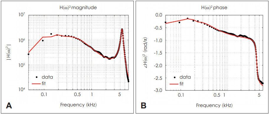
Fig.┬Ā3.
Impulse response [IFFT of H(Žē)2] (A) for the Prony method [9] and fitting estimation by the Prony method (B). IFFT: inverse fast Fourier transform.

Fig.┬Ā4.
Fitting error in %: e(f)=|data-fit|/|data| where f is a frequency. Gustavsen and SemlyenŌĆÖs [8] fitting result shows a lower error rate over the frequency region.
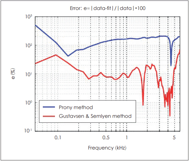
Fig.┬Ā5.
Pole-zero plot of H(Žē)2. Zeros are marked with blue O symbols. Poles are marked with red X symbols.

Fig.┬Ā9.
A simple schematic diagram of a balanced armature receiver system based on energy transformation flow, from an electrical input to an acoustic output. A gyrator is coupling between the electrical part and mechanical part via transduction coefficient T. A delay Žä is represented by a transmission line referring to a pure acoustic delay from mechanic to acoustics.

REFERENCES
1. Robinson SR, Nguyen CT, Allen JB. Characterizing the ear canal acoustic impedance and reflectance by pole-zero fitting. Hear Res 2013;301:168ŌĆō82.


2. Hunt FV. Electroacoustics: the analysis of transduction, and its historical background. Harvard University Press;1954.
3. Kim N, Allen JB. Two-port network analysis and modeling of a balanced armature receiver. Hear Res 2013;301:156ŌĆō67.


4. Wegel RL. Theory of magneto-mechanical systems as applied to telephone receivers and similar structures. J Am Inst Elect Eng 1921;40:791ŌĆō802.

5. Van Valkenburg ME. Network analysis. 2nd ed. Englewood Cliffs, NJ: Prentice-Hall;1964.
6. Carlin HJ, Giordano AB. Network theory: an introduction to reciprocal and nonreciprocal circuits. 1st ed. Englewood Cliffs, NJ: Prentice-Hall;1964.
7. McMillan EM. Violation of the reciprocity theorem in linear passive electromechanical systems. J Acoust Soc Am 1946;18:344ŌĆō7.

8. Gustavsen B, Semlyen A. Rational approximation of frequency domain responses by vector fitting. IEEE Trans Power Delivery 1999;14:1052ŌĆō61.

9. de Prony BR. Essai experimental et Analytique sur les lois de la dilatabilit├® des fluides ├®lastiques et sur celles de la force expansive de la vapeur de lŌĆÖeau et de la vapeur de lŌĆÖalcool, ├Ā diff├®rentes temperatures. J l'Ecole Polytech 1975;1:24ŌĆō76.
10. Marple SL. Digital spectral analysis with applications. Prentice-Hall;1987.


